Motivation
R is a programming language used heavily in statistical and data analytic applications. It is open-source software supported by a large community of academics and practitioners who have created numerous libraries to extend its capabilities. Versions of R are available on all major computing platforms (Windows, Mac OS/X, and Linux) and installation is quite simple. If you are using a laboratory computer, likely it will be installed already. R is nice because you can use it simply for data analytics (reading, plotting, and analyzing data) just by knowing a few function calls. But it is also nice because it is a full-fledged programming language. Many tasks that you think would be ideal for MatLab or Mathematica (vector and matrix operations, for example) are also easily accomplished in R. Most introductory tutorials in R focus on the data analytics. This tutorial focuses on R as a programming language.
Organization
The first procedural language I learned was FORTRAN. Ever since then, when I need to learn a new language I try to find out as quickly as possible how to do what I used to be able to do with FORTRAN: assign and display variables, branch on conditional statements, perform a loop of statements repeatedly, and organize code into functions or subroutines. Once I know those essentials, I can slow down, relax, and begin to learn why the new language might be better than FORTRAN. Let’s use that approach with R.
Getting Started
Install R if it is not already on your computer. (Visit http://cran.r-project.org/).
All installations of R come with a basic graphical user interface, RGUI. There are other user interface choices (such as RStudio) but we assume you are using RGUI for this tutorial.
Launch the R program. You will see a development environment window containing a window called the “R Console.” Inside that window, you will see a prompt where you enter your commands:
Assign and Display Variables
- Enter the command ‘a=50’ followed by the command ‘a’:
## [1] 50The first command assigned the value 50 to the variable ‘a’. The second command caused the value of ‘a’ to be returned to the console for display. The display showed that ‘a’ consists of a single element whose first value (that is what the ‘[1]’ means) is 50.
- Enter the command ‘a/10’:
## [1] 5- This command divides the value of ‘a’ by 10 and returns the result to the console, a single element of value 5. The value of ‘a’ remains unchanged. It will continue to have the value 50 until one of three things happen:
- You enter a new assignment command; for example ‘a=3’; Or,
- You quit the session or close the program; for example, enter ‘q()’; Or,
- You explicitly remove the variable using the command ‘rm(a)’.
- If you refer to a variable that does not exist you will get an error message ‘Object not found.’
rm(a)
a- Variables, also known as objects, have types and structure. To see the type and structure of a variable, use the str() command:
## num 50## chr "hello"As you can see, the type of variable a changed from numeric (“num”) to character (“chr”) by assigning the string value “hello” to the variable. Operations that are possible on one type of object may cause errors when used with another type of object. Try this:
a="hello"
str(a)
a/50This fact puts the responsibility on you, the programmer, to keep track of what type a variable has and to avoid using it incorrectly. Strongly-typed languages, such as C and Java, prevent you from using variables in more than one way. Loosely-typed languages, such as R and Python, give you the freedom to change variable types on the fly.
There are many different types of objects possible in R (and you can create your own). Vectors are extremely useful. Here is how to create a vector:
## [1] 1 2 4 8## [1] 4Here we used the function c() to create a vector of four numbers ranging from 1 to 8. [c() stands for ‘concatenate’: it can be used to concatenate multiple short lists into one long list.] We then used the function length() to check how long a vector we had created.
- There are many ways to create vectors. The syntax
1:4is shorthand for the vector1 2 3 4. Try the following:
##  [1]  1  2  3  4  5  6  7  8  9 10 11 12 13 14 15 16 17 18 19 20 21 22 23 24 25
## [26] 26 27 28 29 30 31 32 33 34 35 36 37 38 39 40 41 42 43 44 45 46 47 48 49 50
Observe that the result is a vector of consecutive numbers from 1 to 50. When displaying the vector, R displays the index of the first element on each display row. That is,
[26]means the second display row begins with the 26th element of the vector.R accepts two methods of assignment:
=(equals) and<-(back arrow, or ‘is replaced by’). The following statements achieve the same thing:
##  [1]  1  2  3  4  5  6  7  8  9 10 11 12 13 14 15 16 17 18 19 20 21 22 23 24 25
## [26] 26 27 28 29 30 31 32 33 34 35 36 37 38 39 40 41 42 43 44 45 46 47 48 49 50## [1] 1 2 3 4 5 6 7 8 9 10 11 12 13 14 15 16 17 18 19 20 21 22 23 24 25
## [26] 26 27 28 29 30 31 32 33 34 35 36 37 38 39 40 41 42 43 44 45 46 47 48 49 50However, in keeping with R tradition, from now on, we will use = only to assign named arguments in lists (see later) and we will use <- for all other assignments. This is what Google [recommends] (https://google-styleguide.googlecode.com/svn/trunk/Rguide.xml). It requires an extra keystroke to type the back arrow (‘<-‘) but there is a shortcut in RStudio (type <ALT>-). To improve readability, we will try to remember to include some extra spaces around the back arrow as well.
- Note what R displays after the following commands:
## [1] 0.2 0.4 0.6 0.8 1.0 1.2 1.4 1.6 1.8 2.0Observe that R took the vector 1:10 and divided each component of the vector by 5. That is important to keep in mind when working with vectors: R will apply operations to each component. You might have expected the answer to be
[1] 1 2Suppose that is the answer you really wanted. Write down the statements, modified using parentheses (()) to get this as the answer.
Branch on Conditionals
The next major requirement of a programming language is the ability to branch on a condition.
- Set a variable equal to a value and then use an ‘if-then-else’ statement to branch on that value. Here is an example you can try:
## [1] "It's a three."Note that the test for equality is the binary operator “==”. If you had used “=” it would have caused an error.
- Suppose you want to execute a block of code based on a condition. In that case, enclose the block of code in curly braces (
{}) and end each statement with a semi-colon (;) or put it on a new line. Try something like the following:
## [1] "It's a three!"
## [1] "It's a three!"
Test your statement with different values of ‘a’. Here is where it is good to know that you don’t need to keep re-typing a statement: Just hit the ‘up’ arrow on your keyboard to return to a statement that you previously typed.
Alternatively, instead of using the semi-colon separator, hit carriage return (the Enter key) to create a new line.
## [1] "It's a three!"
## [1] "It's a three!"
Observe that we used the curly braces after the else statement even though there was only one statement to execute in that case. This is considered good coding style.
- Exercise: On a single line (using curly braces and semi-colons where needed), write down an
if-then-elsestatement that if the variableais greater than 1000 it replaces the value ofawith 1000 and prints the statement “a is too big” and otherwise if the variableais below 10 it replaces the value ofawith 10 and prints the statement “a is too small” and otherwise prints “a ok”. (Be sure to test it with three values: 5, 15, and 1500.)
Perform a Loop of Statements Repeatedly
- Try the following:
## [1] 1
## [1] 2
## [1] 3
## [1] 4
## [1] 5
The variable i acts as an iterator, looping through the elements of the vector 1:5.
- Try the following:
## [1] 2
## [1] 4
## [1] 8
## [1] 16
## [1] 32
That is, to execute a block of code in a loop, combine the for() statement with a block of code enclosed in curly braces ({}) and separated with semi-colons (;) or carriage returns.
- Wherever possible, you should avoid
for()loops in R and take advantage of its much faster vector arithmetic. For example, if you want a vector of powers of two, use the following:
## [1] 2 4 8 16 32- Exercise: write down a
for()loop that will print the value ofsin(x/10)for each value ofxin the rangex=1,2,3,…,10. Use more than one statement inside your loop so that you are forced to use curly braces.
Organize Code into Functions and Subroutines
FORTRAN has the concept of a subroutine which is a block of code that is executed whenever the subroutine is called and a function in which a block of code is executed whenever the function is called and it returns a value computed within the function. In R, a subroutine would simply be a function that does not return a value.
- Try the following:
## [1] 9## [1] 324Observe that the variable name f has been assigned a function definition. From now on, f() can be used as a function (until it is assigned something else, or the session ends, or you enter the remove command rm(f)). It can be confusing to think of variables sometimes having values and other times representing functions. So, from now on, we will refer to the letter f as a symbol. You can list the symbols that have been defined in your session using the command ls() and you can get information about what object is stored in the symbol using the command str(). For example, try typing the following:
## function (x)
##  - attr(*, "srcref")= 'srcref' int [1:8] 1 6 1 21 6 21 1 1
##   ..- attr(*, "srcfile")=Classes 'srcfilecopy', 'srcfile' <environment: 0x0000000012b76158>
The result is not helpful to ordinary programmers like me. Here is what is more helpful:
## function(x){x^2}
## <bytecode: 0x0000000014a02420>
That is, if you type the symbol, R will display what value it holds.
- A subroutine is simply a function that doesn’t return a value. Notice the difference between the following two function definitions:
## [1] 8Observe that, in both cases, the function squares the value of the argument ‘x’ and assigns the result to the symbol ‘result’. However, in the first case, the value is returned from the function by virtue of it being listed (result) as the last statement in the function. In the second case, nothing is returned because the last statement of the function is an assignment statement (result <- x^2). Assignment statements have no return value.
Local-Global Scoping Rules
- It is critical in any programming language to understand its scoping rules. When are variables local or global? Here are some examples that will illustrate R’s scoping rules.
## [1] 25## [1] 4The symbol x is used twice: once outside the definition of the function (x <- 4) and once inside the function (x^2). When the function is called as f(5), the argument of the function is taken to be (x=5) and the value 25 is returned. However, if we check the value of the symbol x, it still has the value 4. That is, the arguments of the function are treated as local variables within the function. But consider the next example:
rm(a)
f = function(x){x^a}
f(3)
This results in an error object 'a' not found. Try it again as follows:
## [1] 9In this example, we removed the symbol a from the session (rm(a)) and defined a function which uses two symbols: x and a. The symbol x is the argument of the function but the symbol a is not assigned anywhere inside the function. When we call the function with argument x=3, we get an error because the symbol a cannot be found. We then assign a value to the symbol ‘a’ (‘a <- 2’) and try again. This time it works: we get the value 9=3^2. This shows us that if R cannot find a symbol defined in a function it will search outside the function (i.e. to the session) to find it.
But now consider this example:
## [1] 9## [1] 3In this example, we defined the symbol a both inside and outside the function. It is assigned the value 2 inside the function and the value 3 outside the function. In this case, a acts like a local variable inside the function: it has no effect on the value of a outside the function.
Suppose we really wanted to change the value of a outside the function as part of the function? How would we do it? We can change the value of symbols outside a function by using a stronger version of assignment operator: Use <<- (double-back arrow).
## [1] 9## [1] 2Here, by using the double-back arrow inside the function, we change the value of the symbol a in the session whenever we call the function f(). This is a dangerous feature! Avoid using it if you can. Use it only if you have complete control over the context in which your program will run.
Function Arguments
- R is beautifully flexible in terms of how you specify arguments for your functions. Here are some examples of that flexibility. Suppose we define a function with one argument but call it with no arguments:
f <- function(x){x^2}
f()
This results in an error: 'x' is missing.
Note that R did not complain about the missing argument until it actually tried to use it as part of a calculation. The error occurred when it tried to evaluate x^2. In other languages, you would have received an error sooner. This is called lazy evaluation and can be quite useful.
Suppose we want to allow the user of our function to call it without any arguments? In that case, we simply need to provide a default value for any argument which can be omitted.
## [1] 0## [1] 16Here we have provided a default value for the argument x (x=0). Now it is possible to call the function both with and without an argument and get a reasonable answer in each case. [Also, note that we used the equals sign to set the default (x=0) and not the back-arrow. This is consistent with our convention to use the equals sign in lists (such as argument lists) and the back-arrow everywhere else.]
R is also beautifully flexible when you have multiple arguments in the argument list. Consider this example:
## [1] 0## [1] 3## [1] 9## [1] 8## [1] 16## [1] 0Here, we have defined a function with two named arguments (x and a) and we have assigned default values to each of these two arguments (x=0 and a=1). As a result, look at all the different ways we can call this function and get valid results! We can call it with no arguments (pow()) because both arguments have defaults. We can call it with just the first argument (pow(3)) because the second argument has a default. We can call it with both arguments, but the order is important (pow(3,2) is different from pow(2,3)). But if we know the names of the arguments, then we can call them in any order provided we assign the values by name (pow(a=2,x=4)). We can also call the function with just the arguments we want and accept the defaults for the other arguments (pow(a=1000)).
You will take advantage of this feature as you learn R. For example, you will begin using some library functions in their very simplest form, accepting all of the defaults. Then, as you learn more of the capabilities of the function, you will take more control and assign values to some of the named arguments to get exactly the result you want.
- Exercise: define a function (you can choose what name to give the function) that accepts two named arguments,
xandxscale, and returns the valuesin(x*xscale). Thexscaleargument should have a default value of 1. Test to make sure that the function can be called with both one and two arguments.
Scripts
To this point, we have demonstrated that R is a fully functioning procedural language, capable of assignment statements, conditional branching, loops, and function definitions. To be really useful as a programming language, however, we have to have a means of saving our code and executing it again at a later time. In R, this is accomplished with scripts. Scripts are simply text files of R statements which can be executed all at once, simply by loading the file.
Using the RGui interface, select
File->New Script. A new window, called “Untitled – R Editor”, should pop up. This is a script editor. You can have many script editors open in the interface at once, but there will always be only one ‘R Console’ window open. The R Console window is where commands are executed. The other windows are just for script editing.In the R Editor window, enter the following statement:
print("Hello, world!")Now, use
File->Save Asand save the file as “HelloWorld.R” in a directory of your choosing. It is conventional to name these text files with the “.R” extension.We would like to load this R script into the session. The command to do this is as follows:
source("HelloWorld.R")This will likely cause an error: No such file or directory.
As you can see, the source command did not work. The reason is that the default R directory did not match the directory in which we saved the file. One way to solve this problem is to be more explicit:
source("C:/Users/pj16/Documents/00pj9/PJ Centric/01 Projects/GDR_Educate/HelloWorld.R")In your case, you would use the file path matching the directory where you saved the file. Observe that the source() command caused the script to be read and executed (the print statement in the script file was executed). Another way to solve the directory problem is to first set the working directory (setwd()) of the R session. Then you can call the source() command in short form:
setwd("C:/Users/pj16/Documents/00pj9/PJ Centric/01 Projects/GDR_Educate/HelloWorld.R")
source("HelloWorld.R")
[Note to Windows users: you can use File Explorer to get directory paths but they will be in the form “C:16\00pj9Centric\01 Projects_Educate” using backslashes (‘’) instead of forward slashes (‘/’). You must convert them to forward slashes for R or insert a backslash in front of each backslash, as in: “C:\Users\pj16\Documents\00pj9\PJ Centric\01 Projects\GDR_Educate”.]
- You will want to do most of your work in the script editors, saving your script files, and only occasionally switching to the R Console to execute something. Let’s create the following simple program and include it in the HelloWorld.R script:
## [1] "Hello, world!"- Save and then load this file into the session again:
source("HelloWorld.R")- Now, in the R console window, we can run the testpow() program we wrote:
## [1] 9
## [1] 8
You should now begin to see how to organize large projects into scripts containing different functions. Functions in one script can call functions in another script provided only that all the scripts are loaded into the R session using the source() command.
- There is one last extremely useful trick to learn about working with scripts. Suppose you are editing a script file and you want to test something in the script file. For example, suppose we want to test the statement `
print(pow(2,3)). In that case, simply select the text you want to execute and hit the ‘r’ key combination.
That has the effect of copying the selected text to R console window and executing it.
This is great for debugging. A related trick is to put the cursor on any line in the script file you want to execute and hit the ‘<CTRL. r’ key combination. That line will be executed and the cursor will advance to the next line. So you can execute several lines in sequence by simply hitting ‘<CTRL r’ repeatedly.
Fun with R
So, R is a procedural language that can do everything an old language like FORTRAN can do. What can it do better? In this section, we will explore some of the data visualization possibilities with R. It will also give us some practice with working with vectors, matrices, and loops.
In what follows, enter all the R statements into your script file so that you can save your work. You do not need to type any of the comment lines (the lines with ‘#’ at the beginning). When the instruction says to execute the code, use the trick described above of selecting all the code and then hitting the key combination ‘
r’. Save your file periodically. Execute the following code:
##   [1]  0.09983342  0.19866933  0.29552021  0.38941834  0.47942554  0.56464247
##   [7]  0.64421769  0.71735609  0.78332691  0.84147098  0.89120736  0.93203909
##  [13]  0.96355819  0.98544973  0.99749499  0.99957360  0.99166481  0.97384763
##  [19]  0.94630009  0.90929743  0.86320937  0.80849640  0.74570521  0.67546318
##  [25]  0.59847214  0.51550137  0.42737988  0.33498815  0.23924933  0.14112001
##  [31]  0.04158066 -0.05837414 -0.15774569 -0.25554110 -0.35078323 -0.44252044
##  [37] -0.52983614 -0.61185789 -0.68776616 -0.75680250 -0.81827711 -0.87157577
##  [43] -0.91616594 -0.95160207 -0.97753012 -0.99369100 -0.99992326 -0.99616461
##  [49] -0.98245261 -0.95892427 -0.92581468 -0.88345466 -0.83226744 -0.77276449
##  [55] -0.70554033 -0.63126664 -0.55068554 -0.46460218 -0.37387666 -0.27941550
##  [61] -0.18216250 -0.08308940  0.01681390  0.11654920  0.21511999  0.31154136
##  [67]  0.40484992  0.49411335  0.57843976  0.65698660  0.72896904  0.79366786
##  [73]  0.85043662  0.89870810  0.93799998  0.96791967  0.98816823  0.99854335
##  [79]  0.99894134  0.98935825  0.96988981  0.94073056  0.90217183  0.85459891
##  [85]  0.79848711  0.73439710  0.66296923  0.58491719  0.50102086  0.41211849
##  [91]  0.31909836  0.22288991  0.12445442  0.02477543 -0.07515112 -0.17432678
##  [97] -0.27176063 -0.36647913 -0.45753589 -0.54402111
Observe that y is a vector of length 100. How can you visualize vectors? The plot function is great for visualizing vectors:
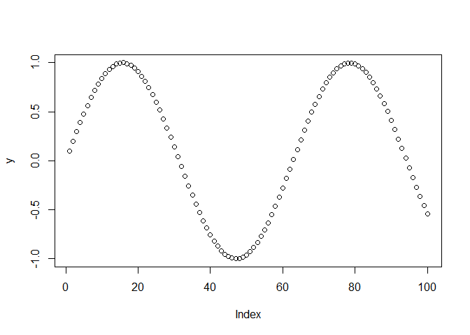
Look for the R Graphics window to see the output of this function.
As you learn more about the defaults for the plot function, you will have greater control over the appearance of your plot. For example, suppose we want to change the color (argument ‘col’) and the title (argument ‘main’) of the plot:
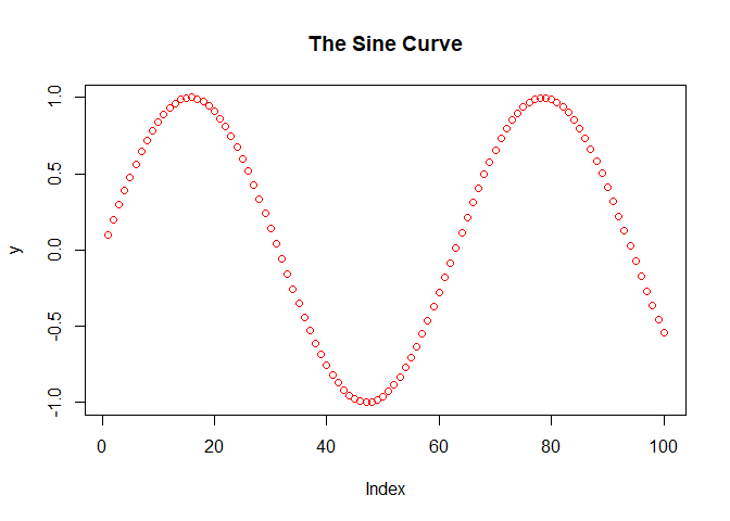
You can learn more about the parameters which control the appearance of the plot at plot
There is a good tutorial on plotting at Intermediate Plotting
- For fun, copy the code below and paste it into your script file and then execute it.
a <- -0.966918
b <- 2.879879
c <- .765145
d <- .744728
n <- 100000
x <- .1
y <- .1
xVector = rep(0,n)
yVector = rep(0,n)
for(i in 1:n) {
newx <- sin(y*b) + c*sin(x*b)
newy <- sin(x*a) + d*sin(y*a)
x <- newx
y <- newy
xVector[i] <- x
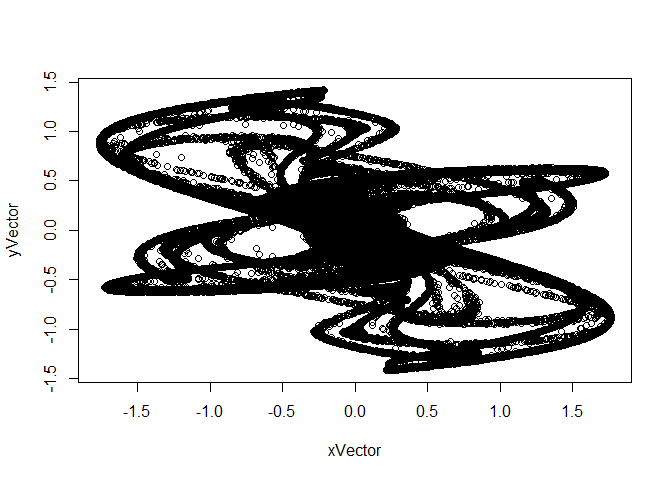
yVector[i] <- y
}This creates two vectors, xVector and yVector, each of length 100,000. What is interesting is to plot them together as a scatterplot:
You can improve the appearance of the plot by replacing certain defaults as follows:
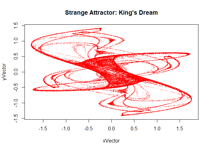
The named argument ‘pch’ refers to the point character, the style of point used. This code came from [Making Simple Fractals in R] (http://hewner.com/2012/10/09/making-simple-fractals-in-r/)
- Next, you can create matrices in a variety of ways. Here is how to create a 10x10 matrix in which each column consists of the numbers 1 through 10:
##       [,1] [,2] [,3] [,4] [,5] [,6] [,7] [,8] [,9] [,10]
##  [1,]    1    1    1    1    1    1    1    1    1     1
##  [2,]    2    2    2    2    2    2    2    2    2     2
##  [3,]    3    3    3    3    3    3    3    3    3     3
##  [4,]    4    4    4    4    4    4    4    4    4     4
##  [5,]    5    5    5    5    5    5    5    5    5     5
##  [6,]    6    6    6    6    6    6    6    6    6     6
##  [7,]    7    7    7    7    7    7    7    7    7     7
##  [8,]    8    8    8    8    8    8    8    8    8     8
##  [9,]    9    9    9    9    9    9    9    9    9     9
## [10,]   10   10   10   10   10   10   10   10   10    10
What is a good way to visualize a matrix? The image() function displays the matrix as a table of colored boxes, where the colors communicate the values of the matrix entries.
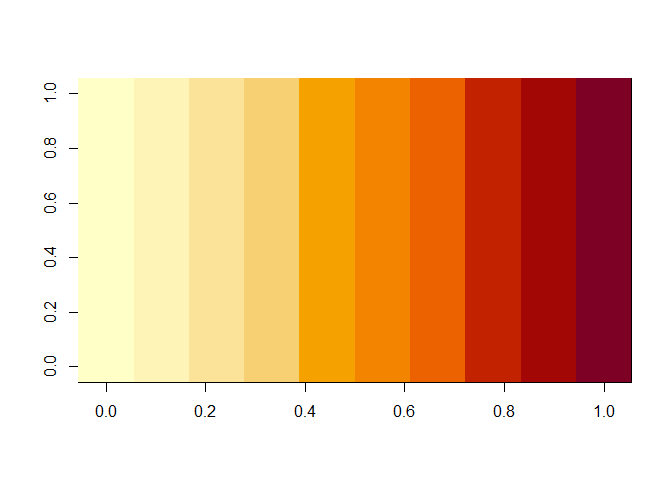
That is not the result I wanted: it has the rows and columns reversed from what I want. So let’s take the transform of the matrix first, using t():
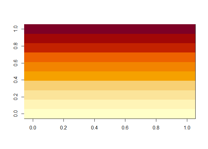
There, that’s better. Now the rows match the vertical dimension and the columns match the horizontal dimension.
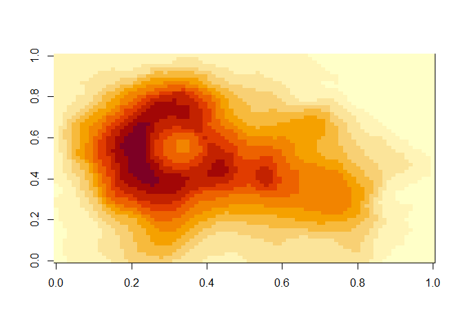
- Rather than create a matrix ourselves, let’s use an interesting matrix that is built into R: the volcano matrix. Enter the following:
volcanoYou should see a display of a pre-defined matrix. It consists of the elevation readings across a grid of different latitude and longitudes of the Maunga Whau volcano, the highest of the New Zealand volcanos.
- Exercise: write the number of rows and columns of this matrix. Hint: use ‘dim(volcano)’ or ‘nrow(volcano)’ and ‘ncol(volcano)’.
So, to visualize this matrix, simply enter the following:
As you can imagine, one of the defaults for this function would be the list of colors to use. We can use a nice color selection function to get a better list:
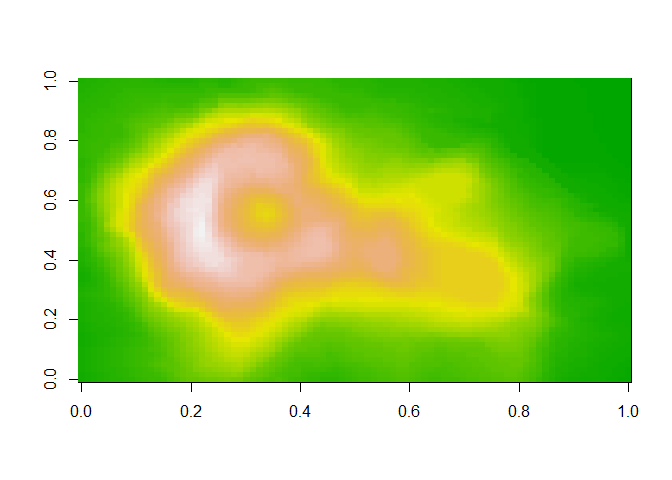
That looks better.
- Using color to view a matrix is nice but it would be even nicer to view the matrix in three dimensions. To do that, we will have to install some other packages for R. Install the following two packages (if you are prompted with a choice of mirror sites, choose one in your country):
## Installing package into 'C:/Users/pj16/Documents/R/win-library/4.0'
## (as 'lib' is unspecified)
## package 'plot3D' successfully unpacked and MD5 sums checked
##
## The downloaded binary packages are in
## C:\Users\pj16\AppData\Local\Temp\Rtmp4gfoYY\downloaded_packagesAnd
## Installing package into 'C:/Users/pj16/Documents/R/win-library/4.0'
## (as 'lib' is unspecified)
## package 'rgl' successfully unpacked and MD5 sums checked
##
## The downloaded binary packages are in
## C:\Users\pj16\AppData\Local\Temp\Rtmp4gfoYY\downloaded_packages- Let’s try the
persp()function onvolcano(it is one of the functions in the plot3D library):
## Warning: package 'plot3D' was built under R version 4.0.5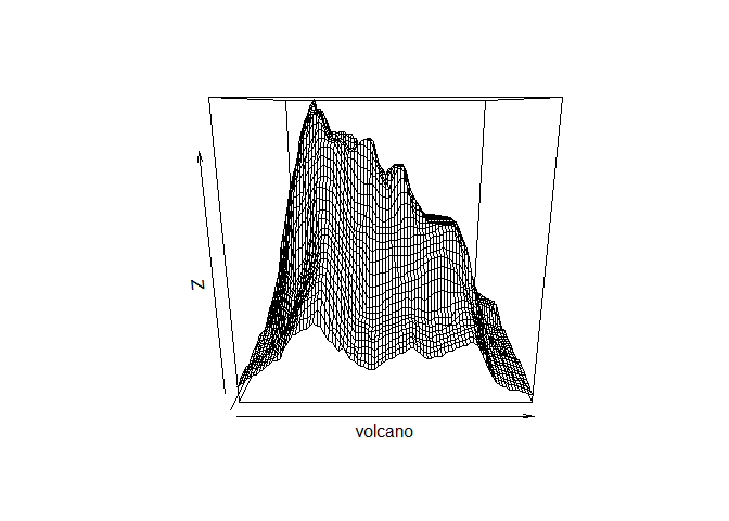
That is interesting but we will have to fuss with the parameters (i.e. read the documentation) to get it to look better:
This is a really interesting matrix!
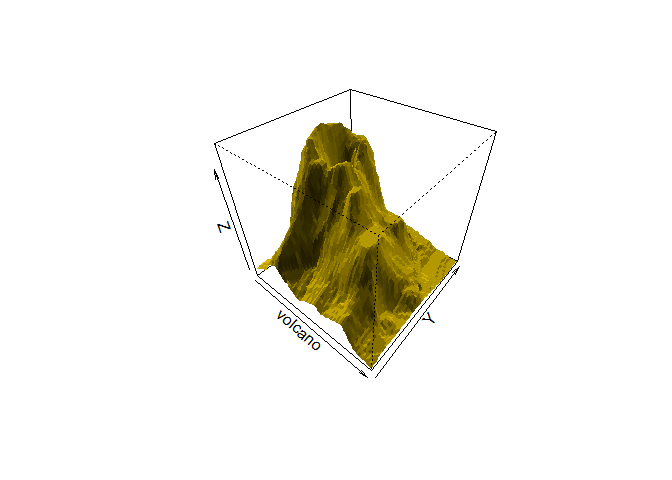
- For the last exercise, simply copy and paste this code into your script editor and then execute it:
## Warning: package 'rgl' was built under R version 4.0.5data(volcano);
z<-3*volcano;
x<-10*(1:nrow(z));
y<-10*(1:ncol(z));
zlim<-range(z);
zlen<-zlim[2]-zlim[1]+1;
colorlut<-terrain.colors(zlen,alpha=0);
col<-colorlut[z-zlim[1]+1];
open3d();## wgl
## 1rgl.surface(x,y,z,color=col,alpha=1,back="lines");
#add the contour map in different color
colorlut <- heat.colors(zlen,alpha=1);
col<-colorlut[z-zlim[1]+1];
rgl.surface(x,y,matrix(1,nrow(z),ncol(z)),color=col,back="fill");This code came from plot 3d topographic map in R.
You should see a window in a separate application that looks like this (use your mouse inside the window to control the view):

More Fun with R
That is the end of this tutorial. But if you like these plots, try running the following commands (one at a time because they take a long time to plot):
source('http://users.utu.fi/attenka/mandelbrot_set.R')source('http://users.utu.fi/attenka/julia_set.R')Visit the following sites to get some interesting code snippets.
Enjoy!