Why Use Databases?
Most R tutorials assume that you are working with a single data file in CSV (Comma Separated Values) format. These CSV files are nice to work with because you can edit them with a spreadsheet program such as Excel. However, for bigger projects and for projects where you are blending reference data with transactional data, it is better to keep all your data in a relational database. Relational databases allow you to better structure your data and establish the relations between reference tables and transactional tables. For example, we may have a table of flight schedules (transactional data) but we want to link it with a table of airports (reference data) to get the names and locations of the flight origins and destinations. And, transactional tables may reference other transactional or transient data. For example, you may want to cross-reference flights with meteorological data.
For these tutorials, we will emphasize the use of relational databases. Most relational databases are defined and manipulated using SQL (the Structured Query Language) although there are slight variations in how the language is implemented for each variant. We will use the SQLite database format because it is the simplest. The only command from SQL we will use explicitly is the SELECT command. We will use R commands to create the database and tables and to insert or append data to the tables.
Load the Relevant Packages
Use the code below to load the packages we will need for this tutorial.
loadPkg <- function(pkgname){
  # require() is the same as library() but returns a logical.
  # character.only= TRUE means pkgname is the name of the package.
  isInstalled <- require(pkgname,character.only = TRUE)
  # If the package has not been installed yet, then install and try again.
  if (!isInstalled) {install.packages(pkgname); library(pkgname,character.only=TRUE)}
}
# We will need the following libraries
loadPkg("DBI")
loadPkg("RSQLite")
Create an SQLite Database file
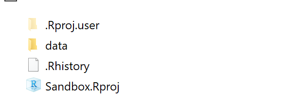
Use your file explorer to create a new sub-directory called “data” within your Sandbox project:
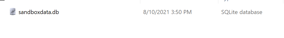
The following code will create an empty SQLite database file within the “data” directory.
# Open an SQLite connection using the filename shown
conn <- dbConnect(RSQLite::SQLite(),"data/sandboxdata.db")
# Close the connection.
dbDisconnect(conn)
Run this code and then check to see that the file was created.
Create a Table from a Data Frame
A typical use case is that we have created a data frame in R and we want to store the data as a table in our database. R comes with many pre-loaded data frames such as mtcars. Suppose we want to save that data in our database.
First, take a look at the mtcars data frame:
##                    mpg cyl disp  hp drat    wt  qsec vs am gear carb
## Mazda RX4         21.0   6  160 110 3.90 2.620 16.46  0  1    4    4
## Mazda RX4 Wag     21.0   6  160 110 3.90 2.875 17.02  0  1    4    4
## Datsun 710        22.8   4  108  93 3.85 2.320 18.61  1  1    4    1
## Hornet 4 Drive    21.4   6  258 110 3.08 3.215 19.44  1  0    3    1
## Hornet Sportabout 18.7   8  360 175 3.15 3.440 17.02  0  0    3    2
## Valiant           18.1   6  225 105 2.76 3.460 20.22  1  0    3    1
# Open an SQLite connection using the filename shown
conn <- dbConnect(RSQLite::SQLite(),"data/sandboxdata.db")
# First delete the table if it already exists
if (dbExistsTable(conn,"mtcars")) dbRemoveTable(conn,"mtcars")
# Create a blank table called "mtcars" using the columns of the mtcars data frame.
dbCreateTable(conn,"mtcars",mtcars)
# Now append the data from mtcars into the database table
dbAppendTable(conn,"mtcars",mtcars)## [1] 32Always remember to use dbDisconnect to close your connection to your database. The reason is that your computer can only have a small number of database connections open at any one time. If you run out of available connections, you may have to restart your computer.
Access Our Data
Now that we have created our database with a sample table and data, let’s see how to access that data.
First, suppose we want to see a list of all the tables in our database:
# Open an SQLite connection using the filename shown
conn <- dbConnect(RSQLite::SQLite(),"data/sandboxdata.db")
# List all the tables in the database
dbListTables(conn)
isclosed <- dbDisconnect(conn) # dbDisconnect() returns TRUE if successful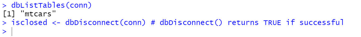
For a given table, suppose we want to see the list of fields (columns) for that table:
##  [1] "mpg"  "cyl"  "disp" "hp"   "drat" "wt"   "qsec" "vs"   "am"   "gear"
## [11] "carb"More commonly, we will want to read the data from our table back into a data frame. That is where the SELECT command comes in.
conn <- dbConnect(RSQLite::SQLite(),"data/sandboxdata.db")
newdata <- dbGetQuery(conn,"SELECT * FROM mtcars")
isclosed <- dbDisconnect(conn) # dbDisconnect() returns TRUE if successful
head(newdata)
## mpg cyl disp hp drat wt qsec vs am gear carb
## 1 21.0 6 160 110 3.90 2.620 16.46 0 1 4 4
## 2 21.0 6 160 110 3.90 2.875 17.02 0 1 4 4
## 3 22.8 4 108 93 3.85 2.320 18.61 1 1 4 1
## 4 21.4 6 258 110 3.08 3.215 19.44 1 0 3 1
## 5 18.7 8 360 175 3.15 3.440 17.02 0 0 3 2
## 6 18.1 6 225 105 2.76 3.460 20.22 1 0 3 1The string “SELECT * FROM mtcars” is an SQL query command that is passed to the database using the function dbGetQuery(). It is executed on the database and the result is returned as a data frame. The asterisk (’*’) indicates that you want all the fields returned. If you just wanted a subset of the columns, say “mpg” and “disp”, you would list them explicitly as in this example:
conn <- dbConnect(RSQLite::SQLite(),"data/sandboxdata.db")
newdata <- dbGetQuery(conn,"SELECT mpg,disp FROM mtcars")
isclosed <- dbDisconnect(conn) # dbDisconnect() returns TRUE if successful
head(newdata)
## mpg disp
## 1 21.0 160
## 2 21.0 160
## 3 22.8 108
## 4 21.4 258
## 5 18.7 360
## 6 18.1 225Aside: What Happened to the Car Names?
We can see that the names of the cars did not get stored in the database table. The reason is that the cars appear as row names in the original data frame mtcars but the commands dbCreateTable() and dbAppendTable ignore row names of dataframes. We can fix that by converting the rownames to a column in the data frame. This is shown below.
##    mpg cyl disp  hp drat    wt  qsec vs am gear carb             names
## 1 21.0   6  160 110 3.90 2.620 16.46  0  1    4    4         Mazda RX4
## 2 21.0   6  160 110 3.90 2.875 17.02  0  1    4    4     Mazda RX4 Wag
## 3 22.8   4  108  93 3.85 2.320 18.61  1  1    4    1        Datsun 710
## 4 21.4   6  258 110 3.08 3.215 19.44  1  0    3    1    Hornet 4 Drive
## 5 18.7   8  360 175 3.15 3.440 17.02  0  0    3    2 Hornet Sportabout
## 6 18.1   6  225 105 2.76 3.460 20.22  1  0    3    1           Valiant
Now let’s retrace our steps with this replacement data frame.
# Open an SQLite connection using the filename shown
conn <- dbConnect(RSQLite::SQLite(),"data/sandboxdata.db")
# First delete the table if it already exists
if (dbExistsTable(conn,"mtcars")) dbRemoveTable(conn,"mtcars")
# Create a blank table called "mtcars" using the columns of the olddata data frame.
dbCreateTable(conn,"mtcars",olddata)
# Now append the data from olddata into the database table
dbAppendTable(conn,"mtcars",olddata)
## [1] 32Now, read the data from the database and see if it has the car names.
conn <- dbConnect(RSQLite::SQLite(),"data/sandboxdata.db")
newdata <- dbGetQuery(conn,"SELECT names,mpg,disp FROM mtcars")
isclosed <- dbDisconnect(conn) # dbDisconnect() returns TRUE if successful
head(newdata)
## names mpg disp
## 1 Mazda RX4 21.0 160
## 2 Mazda RX4 Wag 21.0 160
## 3 Datsun 710 22.8 108
## 4 Hornet 4 Drive 21.4 258
## 5 Hornet Sportabout 18.7 360
## 6 Valiant 18.1 225Get Selective With Your Queries
The SELECT statement in SQL is powerful. By adding certain clauses to the statement you can customize what result is returned. For example, suppose you wanted only a small number of rows of the table returned, for test purposes. Here we ask for just three rows using the LIMIT clause:
conn <- dbConnect(RSQLite::SQLite(),"data/sandboxdata.db")
newdata <- dbGetQuery(conn,"SELECT names,mpg,disp FROM mtcars LIMIT 3")
isclosed <- dbDisconnect(conn) # dbDisconnect() returns TRUE if successful
# We display the whole result and not just the head:
newdata
## names mpg disp
## 1 Mazda RX4 21.0 160
## 2 Mazda RX4 Wag 21.0 160
## 3 Datsun 710 22.8 108Or, suppose we wanted to see the top 3 fuel efficient cars:
conn <- dbConnect(RSQLite::SQLite(),"data/sandboxdata.db")
# ORDER BY ... DESC sorts the result in descending order of the specified field
newdata <- dbGetQuery(conn,"SELECT names,mpg,disp FROM mtcars ORDER BY mpg DESC LIMIT 3")
isclosed <- dbDisconnect(conn) # dbDisconnect() returns TRUE if successful
# We display the whole result and not just the head:
newdata
## names mpg disp
## 1 Toyota Corolla 33.9 71.1
## 2 Fiat 128 32.4 78.7
## 3 Honda Civic 30.4 75.7Or, suppose we wanted to see all 4-carburetor models:
conn <- dbConnect(RSQLite::SQLite(),"data/sandboxdata.db")
# the WHERE clause specifies conditions the row must match
newdata <- dbGetQuery(conn,"SELECT names,mpg,disp FROM mtcars WHERE carb=4")
isclosed <- dbDisconnect(conn) # dbDisconnect() returns TRUE if successful
# We display the whole result and not just the head:
newdata
## names mpg disp
## 1 Mazda RX4 21.0 160.0
## 2 Mazda RX4 Wag 21.0 160.0
## 3 Duster 360 14.3 360.0
## 4 Merc 280 19.2 167.6
## 5 Merc 280C 17.8 167.6
## 6 Cadillac Fleetwood 10.4 472.0
## 7 Lincoln Continental 10.4 460.0
## 8 Chrysler Imperial 14.7 440.0
## 9 Camaro Z28 13.3 350.0
## 10 Ford Pantera L 15.8 351.0There is lots more you can do with the SELECT statement but that is enough to get you started.
Summary
- Relational databases allow us to link transactional data with reference data.
- Most relational databases are manipulated using SQL (the Structured Query Language).
- SQLite is a simple relational database suitable for many projects.
- The DBI and RSQLite packages provide a simple interface to SQLite databases.
- You connect to a database with dbConnect() and disconnect with dbDisconnect().
- Remember to close every connection you open.
- You can create and connect to an SQLite database with dbConnect().
- Useful functions: dbExistsTable(),dbRemoveTable(),dbCreateTable(), dbAppendTable(), and dbGetQuery().
- The SQL SELECT command is powerful: use clauses LIMIT, ORDER BY, and WHERE to refine your query result.