Motivation: Construct an Airports Table
The problem we would like to solve is to create and populate a table in our database for airports. For each airport in the table we would like to know its name and geographical coordinates. At the very least, we would like to be able to plot these locations on a map.
Such data exist on the web but we would like to compile a subset of the data for our research purposes and store it in a local database.
We will demonstrate the technique using the Falling Rain website. If you intend to use their data for commercial purposes, please contact them directly. Our usage here is educational.
Three Levels to the Data: World, Country and Airports
The Falling Rain data are organized into three levels. At their Global Gazetteer you see a world list of links to individual countries.
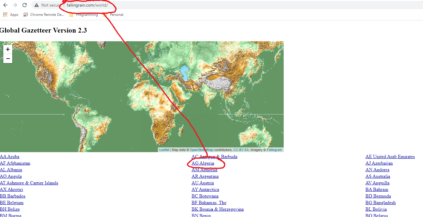
If you click on one of the country links, for example “AG Algeria”, you are taken to page for that country.
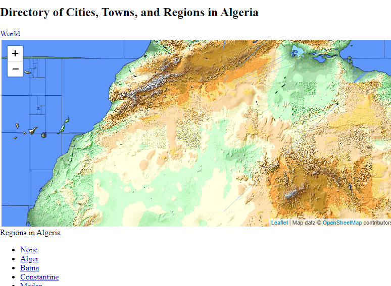
Scroll down the country page and you will find a link to the airports data.
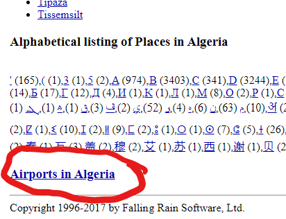
Click on the “Airports in …” link and you will be taken to a web page listing the airports in that selected country.
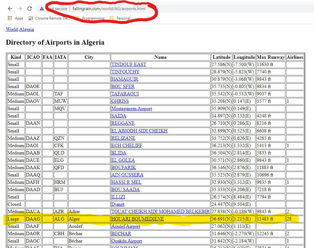
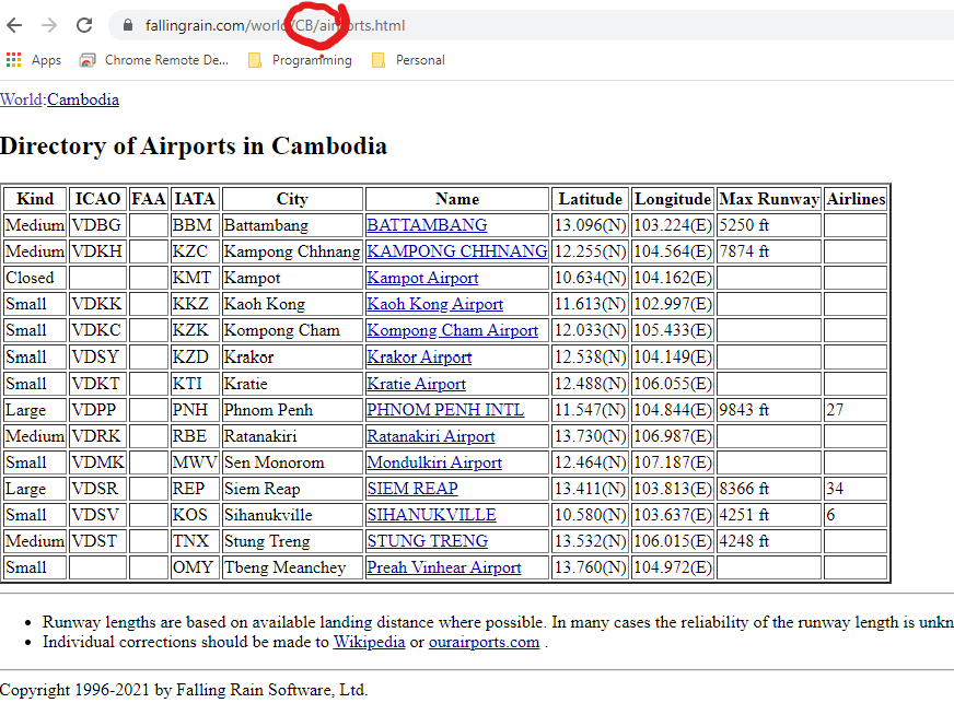
This table has the data we are looking for (ICAO and IATA codes, airport name, city name, latitude and longitude) but more rows than we likely will want. Let’s plan on scraping just the “Large” airports such as Houari Boumediene, as highlighted.
Note that there is a pattern in the URL (“fallingrain.com/world/AG/airports.html”). To get to the airport table for any country we can likely just enter the URL, “fallingrain.com/world/XX/airports.html”, where “XX” is the two character country code. For example, to get to the page for Cambodia (“CB”) we would use the URL “fallingrain.com/world/CB/airports.html”.
Problem Statement: Extract Country Codes and Airports
To summarize, our goal is to develop two tables in our local database: a listing of two character country codes and, for a sample of country codes, a listing of the large airports in each of those countries with details for ICAO and IATA codes, airport name, city name, latitude and longitude. We will call one table “countrycodes” and the other table “airports”.
Background: Structure of HTML Documents
Documents on the web are accessible as HTML (HyperText Markup Language) format files. These files organize the text and images to display into nodes and the nodes can be nested inside other nodes. Each node has a markup tag at beginning and the end (for example <table> starts a table node and </table> ends it). There can be many, many levels of nesting, so we refer to this as tree-structured data. This is illustrated in the following diagram:
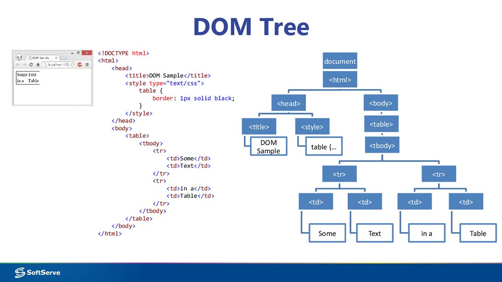
(Source: “https://ppt-online.org/83335”)
On the left you see a simple HTML document file with the nesting clearly indicated using indented lines. At the deepest level you see text (“Some”, “Text”,“in a”, “Table”) nested within individual <td> and </td> tags. Given an HTML file, therefore, our task will be to locate the deepest level nodes which contain the data we are interested in and then extract that data.
Where are the Data?
Before we see how to perform our task programmatically, let’s look at the HTML documents at Falling Rain to locate the data we want.
Go back to Global Gazetteer but this time hit <ctrl>u on your keyboard to view the raw html file for this page. (Alternatively, use your Firefox menu to view “More tools->Page Source” or your Chrome menu to view “More tools->Developer tools”.)
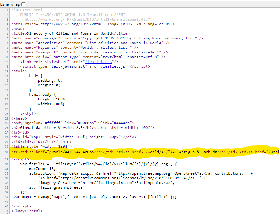
We spot the list of countries inside <td></td> tags. Groups of those tags are nested inside <tr></tr> tags (organizing the data into rows). All of those rows are nested inside a pair <table></table>. You would have to scroll all the way to the right to spot the closing </table> tag, but it is there. Observe that this is not the only such <table></table> pair on the page: it is the second of two tables. That is how we will identify it.
Similarly, if we visit URL (“fallingrain.com/world/AG/airports.html”) and hit <ctrl>u we can examine the HTML for a typical airports page.
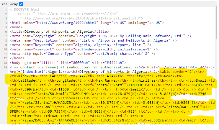
On this page there is a single <table></table> node. The first row of the table, marked with <tr></tr> is the header row. Every row after that contains the data we are looking for.
We are ready to write code.
Create a New Script
Our intent is that you copy all the code from this tutorial into a separate script file and execute the code from there. Call the file “scrapeAirports.R”, or something, and save it in the Sandbox project directory you created in the “Introduction to RStudio” tutorial. That directory should also contain the sub-directory “data” with the “sandboxdata.db” database file created in the “Introduction to Databases” tutorial.
Load the Relevant Packages
Use the code below to load the packages we will need for this tutorial. (Copy this code to your script file “scrapeAirports.R”)
loadPkg <- function(pkgname){
  # require() is the same as library() but returns a logical.
  # character.only= TRUE means pkgname is the name of the package.
  isInstalled <- require(pkgname,character.only = TRUE)
  # If the package has not been installed yet, then install and try again.
  if (!isInstalled) {install.packages(pkgname); library(pkgname,character.only=TRUE)}
}
# We will need the following libraries
loadPkg("DBI")
loadPkg("RSQLite")
loadPkg("stringr")  # For string concatentation (str_c) and other nice string manipulation
loadPkg("rvest")    # For processing HTML documents
loadPkg("dplyr")    # For post-processing the data
Build and Test a Scraping Function
Add the following code to your script file.
getCountryAirports <- function(countrycode){
  # Use the str_c() concatenate function to create the URL customized for the country code
  url <- str_c("http://www.fallingrain.com/world/",countrycode,"/airports.html")
  url
}

test <- function(){
  countrycode <- "AG"
  result <-  getCountryAirports(countrycode)
  print(result)
}
Run the script (execute all lines) and then, in the console window, enter the command “test()”. You should see the following.

This demonstrates that we can programmatically generate a valid url string.
Modify the getCountryAirports() function as follows (keep the test function unchanged).
getCountryAirports <- function(countrycode){
  # Use the str_c() concatenate function to create the URL customized for the country code
  url <- str_c("http://www.fallingrain.com/world/",countrycode,"/airports.html")
  # Use rvest to read the html document at this url
  airportpage <- read_html(url)
  airportpage
}
Run the script (execute all lines) and then, in the console window, enter the command “test()”. You should see the following.

At the highest level, the html document at this URL has two nodes: a <head></head> node and <body></body>. We know that the data we want is somewhere in the body node. We know that it is within a table node and that there is only one table on the page. The rvest has a variety of tools to locate and extract the data you want. In this case, two commands suffice. Replace the getCountryAirports() function as follows (keep the test function unchanged).
getCountryAirports <- function(countrycode){
  # Use the str_c() concatenate function to create the URL customized for the country code
  url <- str_c("http://www.fallingrain.com/world/",countrycode,"/airports.html")
  # Use rvest to read the html document at this url
  airportpage <- read_html(url)
  # Find the first occurrence of a table node on the page
  tablenode <- html_node(airportpage,"table")
  # rvest understands html tables so it is easy to convert to a data frame
  dfnode <- html_table(tablenode)
  # return the data frame
  dfnode
}
Run the script (execute all lines) and then, in the console window, enter the command “test()”. You should see the following. 
Success! We have extracted a data frame of airports for a country code of our choosing. However, before saving this to our database we would like to filter and simplify the data for our purposes.
Wrangle the Data
The tidyverse packages in R are fantastic for wrangling data into the form you want. We will use a few functions from the dplyr package and the stringr package (both are part of the tidyverse) to filter and simplify the data.
We want to accomplish the following:
- Eliminate all rows except for the “Large” airports.
- Remove the “Kind” column (since we only care about one kind).
- Add the country code as a column
- Drop the “FAA” and “Max Runway” columns.
- Strip the hemisphere designators (“(N)”,“(S)”,“(E)”,“(W)”) since the sign makes them redundant.
- Convert the resulting latitude and longitude columns to numeric (double) data types.
- Convert the tibble back to a data frame
Here is a verbose way of doing it:
getCountryAirports <- function(countrycode){
  # Use the str_c() concatenate function to create the URL customized for the country code
  url <- str_c("http://www.fallingrain.com/world/",countrycode,"/airports.html")
  # Use rvest to read the html document at this url
  airportpage <- read_html(url)
  # Find the first occurrence of a table node on the page
  tablenode <- html_node(airportpage,"table")
  # rvest understands html tables so it is easy to convert to a data frame
  dfnode <- html_table(tablenode)
  # Filter out rows that do not match "Large" kinds of airports. Remember to use "==".
  dfnode <- filter(dfnode,Kind=="Large")
  # Remove the "Kind" column
  dfnode <- select(dfnode,-Kind)  # That is, select all columns except the Kind column
  # Add the country code
  dfnode <- mutate(dfnode,Country=countrycode)
  # Remove the  "FAA", "Max Runway" columns
  dfnode <- select(dfnode,-FAA,-"Max Runway") # Quote 'Max Runway' because it has a space
  # Strip hemisphere designator from Latitude
  dfnode <- mutate(dfnode,Latitude=str_replace(Latitude,"\\(.\\)","")) # See tutorial on string manipulation
  # Strip hemisphere designator from Longitude
  dfnode <- mutate(dfnode,Longitude=str_replace(Longitude,"\\(.\\)","")) # See tutorial on string manipulation
  # Convert Latitude to double
  dfnode <- mutate(dfnode,Latitude=as.double(Latitude))
  # Convert Longitude to double
  dfnode <- mutate(dfnode,Longitude=as.double(Longitude))
  # Convert from tibble back to data frame
  dfnode <- as.data.frame(dfnode)
  # return the data frame
  dfnode
}
Run the script (execute all lines) and then, in the console window, enter the command “test()”. You should see the following. 
A More Elegant Syntax: Piping
The tidyverse packages support piping. That is, you can pass the output of a tidyverse function as the first input to another tidyverse function. The piping operator is “%>%” (use shortcut <ctrl><shift>m on your keyboard in RStudio). So we can accomplish the entire pipeline of data wrangling as follows:
getCountryAirports <- function(countrycode){
  # Use the str_c() concatenate function to create the URL customized for the country code
  url <- str_c("http://www.fallingrain.com/world/",countrycode,"/airports.html")
  # Use rvest to read the html document at this url
  airportpage <- read_html(url)
  # Find the first occurrence of a table node on the page
  tablenode <- html_node(airportpage,"table")
  # rvest understands html tables so it is easy to convert to a data frame
  dfnode <- html_table(tablenode) %>%
  # Filter out rows that do not match "Large" kinds of airports. Remember to use "==".
            filter(Kind=="Large")  %>%
  # Remove the "Kind" column
            select(-Kind)  %>%  # That is, select all columns except the Kind column
  # Add the country code
            mutate(Country=countrycode) %>%
  # Remove the  "FAA", and "Max Runway" columns
            select(-FAA,-"Max Runway") %>%  # Quote 'Max Runway' because it has a space
  # Strip hemisphere designator from Latitude
            mutate(Latitude=str_replace(Latitude,"\\(.\\)",""))  %>% # See tutorial on string manipulation
  # Strip hemisphere designator from Longitude
            mutate(Longitude=str_replace(Longitude,"\\(.\\)",""))  %>% # See tutorial on string manipulation
  # Convert Latitude to double
            mutate(Latitude=as.double(Latitude)) %>%
  # Convert Longitude to double
            mutate(Longitude=as.double(Longitude)) %>%
  # Convert from tibble back to data frame
            as.data.frame()
  # return the data frame
  dfnode
}
Observe that we added the pipe operator “%>%” to the end of each row, removed “dfnode” as the first argument in each function, and made it into one single assignment statement “dfnode <- …”. You will find piping to be a very natural way to think about data wrangling.
Create the Airports Table in the Database
Review the tutorial “Introduction to Databases” before this next step. Add the following function to your script.
createAirportsTable <- function(){
  # Get a sample of the data we want to add
  countrycode = "AG" # We know this works
  airports <- getCountryAirports(countrycode)
  # Open an SQLite connection using the filename shown
conn <- dbConnect(RSQLite::SQLite(),"data/sandboxdata.db")
# First delete the table if it already exists
if (dbExistsTable(conn,"airports")) dbRemoveTable(conn,"airports")
# Create a blank table called "airports" using the columns of the airports data frame.
dbCreateTable(conn,"airports",airports)
# (We will not use the data from our data frame, only the column information)
# Prove that the table was created
print(dbListTables(conn))
# Close the connection.
dbDisconnect(conn)
}
Execute your script and then enter “createAirportsTable()” in the console window. The new table should be listed.

The “airports” table is new. The “mtcars” table was created in the earlier tutorial on databases.
Append Airports Data to the Airports Table
We will be looping over each country, extracting the airports for that country and then appending them to the airports database table. For that purpose we create a function to append data for a single country code.
appendCountryAirports <- function(countrycode) {
  airports <- getCountryAirports(countrycode)
  # Open an SQLite connection using the filename shown
  conn <- dbConnect(RSQLite::SQLite(),"data/sandboxdata.db")
  # Append the data to the airports table
  dbAppendTable(conn,"airports",airports)
  # Close the connection.
  dbDisconnect(conn)
}
Repeat the Process: Build a Country Codes Table
You’ve seen the basic process now. We will repeat our steps to extract a list of country codes from the Global Gazetter page. The main difference here is that page contained two tables marked by <table></table> tags and the data we want is in the second table. Look for how we select just that table. The data wrangling portion is a little different here because the table was formatted in an “untidy” way: instead of three columns we had to reform it into one long column.
buildCountryCodesTable <- function(){
  url <- "https://www.fallingrain.com/world/"
  worldpage <- read_html(url)
  # Find all occurrence of a table node on the page
  tablenodes <- html_nodes(worldpage,"table")
  # Use just the second table
  tablenode <- tablenodes[2]
  # Convert to a tibble, actually a list of tibbles: extract the first one
  dfnode <- html_table(tablenode) [[1]]

  # Treat each column as a separate data frame and bind the rows together into a single column
  df1 <-  as.data.frame(dfnode$X1) %>% rename(country="dfnode$X1")
  df2 <- as.data.frame(dfnode$X2) %>% rename(country="dfnode$X2")
  df3 <- as.data.frame(dfnode$X3)  %>% rename(country="dfnode$X3")
  dfnodenew <- df1 %>% rbind(df2) %>% rbind(df3)

  # Split the column into country code and name
  dfnodenew$countrycode <-  str_sub(dfnodenew$country,start=1L,end=2L)
  dfnodenew$name <- str_sub(dfnodenew$country,start=4L,end=-1L)

  # Drop the country column and eliminate rows with NA countrycode
  dfnodenew <-dfnodenew %>%  select(-country) %>% filter(!is.na(countrycode))

  conn <- dbConnect(RSQLite::SQLite(),"data/sandboxdata.db")
  # First delete the table if it already exists
  if (dbExistsTable(conn,"countrycodes")) dbRemoveTable(conn,"countrycodes")
  # Create a blank table called "countrycodes" using the columns of the dfnodenew data frame.
  dbCreateTable(conn,"countrycodes",dfnodenew)
  # Append the data we just extracted
  dbAppendTable(conn,"countrycodes",dfnodenew)
  # Prove that the table was created
  print(dbListTables(conn))
  # Close the connection.
  dbDisconnect(conn)

}
Execute your script and then enter “buildCountryCodesTable()” in the console window. The new table should be listed.

Putting It All Together
Our final function will use a SELECT query to select just two (2) country codes and extract the airports for these two codes, saving them to the database. You could remove the WHERE clause if you wanted a table of all large airports.
buildAirportsTable <- function(){
  # First create the airports table
  createAirportsTable()
  # Then, build the Country Codes table
  buildCountryCodesTable()
  # Then get three country codes
  conn <- dbConnect(RSQLite::SQLite(),"data/sandboxdata.db")
  # Let's pick France and Algeria
  query <- "SELECT countrycode FROM countrycodes WHERE countrycode='AG' OR countrycode='FR'"
  result <- dbGetQuery(conn,query )
  print(result)
  dbDisconnect(conn)
  # Loop over all the countrycodes in the result and append the airports for each code to the airports table
  for (i in 1:nrow(result)){
    countrycode <- result$countrycode[i]
    appendCountryAirports(countrycode)
  }
  # Now to test the result, query the airports table
  conn <- dbConnect(RSQLite::SQLite(),"data/sandboxdata.db")
  result <- dbGetQuery(conn,"SELECT * FROM airports")
  dbDisconnect(conn)
  print(result)

}
If you were to execute this new script and then enter “buildAirportsTable()” in the console window, you would see the following:
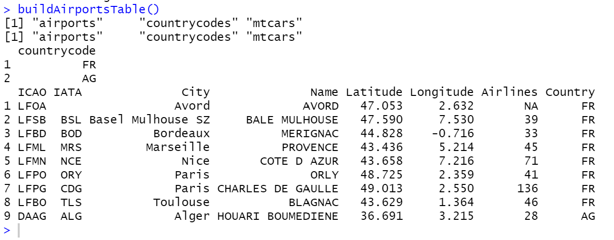
Success! We have a way now to build a database table of airports.
Summary
- Webpages are HTML documents which organize text and images using tags into tree-structured nodes.
- The
rvestpackage can be use to read HTML files from the web and locate nodes of interest. - If the data you seek is in an HTML table, then the function
html_table()can convert it into a data frame. - Once you have your data frame you can use the
dplyrandstringpackages to wrangle the data into the form you want. - The
tidyversepackages likedplyrsupport piping which turns your data wrangling process into a pipeline. - Use the
DBIpackage to store your data frames in a database.