Motivation
Some websites offer data services permitting you to stream live data into your applications. An example is the Open Sky Network.
 This site collects and serves live ADS-B data from volunteer and governmental listening sites around the world. Aircraft using Automatic Dependent Surveillance-Broadcast (ADS-B) record their position determined by satellite navigation and periodically broadcast it over the publicly accessible 1090 MHz radio frequency channel. ADS-B receivers are inexpensive and easy to install. If you live near a corridor of high air traffic, consider installing one, with the appropriate permissions, and joining the Open Sky Network of listeners.
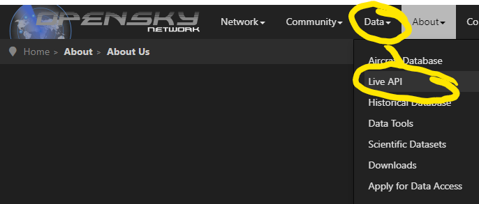
The Open Sky Network offers several ways to access their data for research purposes. In this session, we demonstrate how to both access live ADS-B data and archive it in your local database. In the next session, we will show how to animate a display of the aircraft movements we capture. The method to access the live data through an Application Programming Interface (API) is documented under the Open Sky Network menu item Data->Live API, shown below.
Load the Packages We Will Use
Copy the following code to a new script file in your sandbox folder and execute it to load the packages we will be using.
loadPkg <- function(pkgname){
  # require() is the same as library() but returns a logical.
  # character.only= TRUE means pkgname is the name of the package.
  isInstalled <- require(pkgname,character.only = TRUE)
  # If the package has not been installed yet, then install and try again.
  if (!isInstalled) {install.packages(pkgname); library(pkgname,character.only=TRUE)}
}
# We will need the following libraries
loadPkg("DBI")  # For database operations
loadPkg("RSQLite") # For connection to SQLite databases
loadPkg("stringr")  # For string concatentation (str_c) and other nice string manipulation
loadPkg("dplyr")    # For post-processing the data
loadPkg("httr") # For retrieving internet pages
loadPkg("rjson") # For converting json objects to R objects
loadPkg("leaflet") # For displaying geographical data
Form the URL to Access the API
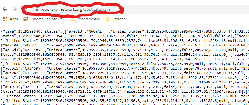
We will use the OpenSky REST API. Using this approach, we access the API of Open Sky Network by issuing a GET command over the internet. The httr package enables us to issue these commands from R. The content of the GET command is a URL string. The first part of the string is https://opensky-network.org/api/states/all?. Try pasting this string into your browser search bar. After a few seconds delay, you should receive a big block of text back, as shown below.
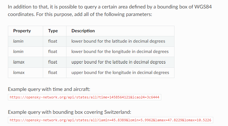
When you end the URL with “all?” the API will return the most recent worldwide ADS-B data. You can refine the query by adding clauses after the question mark (“?”). You can request a range of historical times, specific aircraft, or specific regions. For example, from the RESP API documention:
As suggested, try copying and pasting the following URL’s into your browser search bar to see what is returned.
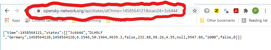
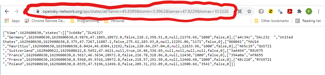
https://opensky-network.org/api/states/all?time=1458564121&icao24=3c6444(a specific time in history, and aircraft)https://opensky-network.org/api/states/all?lamin=45.8389&lomin=5.9962&lamax=47.8229&lomax=10.5226(current activity over Switzerland)
You should see the following for the first URL,
and something like this for the second URL:
Let’s create a general purpose function which can query the OpenSky API for a string of clauses (the argument query we provide). Copy and paste this code into your sandbox script. This will return the block of text as a JSON string. (JSON is a standard for conveying data in human-readable form.)
getOpenSkyData <- function(query){
  url <- 'https://opensky-network.org/api/states/all'
  urlquery <- str_c(url,query,sep="?")
  #print(urlquery) # For debugging: comment this line out when fully debugged
  response <- GET(urlquery)  # from the httr package
  # Extract the body of the response
  # The result should be a character vector of length 1 containing a json string
  jsonString <- content(response,as="text")
  jsonString
}
Do not execute this function yet. We will write a few more functions and then test them all at once. (See Test the Functions below.)
Wrangle the Data into Suitable Database Form
The function we created in the previous section, getOpenSkyData(), returns a JSON string. Our next task is to interpret this string and re-form it into a data frame. Once we have it in the form of a data frame it will be easy to store it in our local database.
For data wrangling such as this, we recommend the dplyr package in R. There are many great tutorials online to learn this package. We recommend R for Data Science by Wickham and Grolemund. We use the mutate() function to modify the data types of the columns in our data frame. Copy and paste the following code into your sandbox script.
extractAircraftStates <- function(jsonString){
  # Convert the json string to an R object
  openskyresponse <- fromJSON(jsonString)
  currenttime <-  openskyresponse$time  # This will be UNIX format time (number of seconds since 1/1/1970)
  numstates <- length(openskyresponse$states)
  # Create a variable to hold the resulting data frame
  dfAircraftStates <- NULL
  # Anticipate the column names (from https://opensky-network.org/apidoc/rest.html)
  statenames <- c("icao24","callsign","origin_country","time_position","last_contact","longitude","latitude","baro_altitude","on_ground","velocity","true_track","vertical_rate","sensors","geo_altitude","squawk","spi","position_source")
  i <- 1 # For debugging
  # Loop over each aircraft
  for (i in 1:numstates){
    # Get aircraftstate
    aircraftstate <- openskyresponse$states[[i]]
    # Some of the fields in aircraftstate can be NULL: convert NULL's to NA's.
    numfields <- length(aircraftstate)
    for (j in 1:numfields){
      aircraftstate[[j]] <- ifelse(is.null(aircraftstate[[j]]),NA,aircraftstate[[j]])
    }
    # Convert the list to a vector
    aircraftstate <- unlist(aircraftstate)
    # Apply the column names
    names(aircraftstate) <- statenames
    # Convert the vector to a named list
    aircraftstate <- as.list(aircraftstate)
    # Convert the vector to a data frame (with a single row)
    aircraftstate <- as.data.frame(aircraftstate)
    # Append the row to the big data frame
    if (i==1) dfAircraftStates <- aircraftstate else dfAircraftStates <- rbind(dfAircraftStates,aircraftstate)
  }
  # Get column names of fields which should be integer
  integerfields <- c("time_position","last_contact","position_source")
  # Convert approriate columns to integer
  dfAircraftStates <- mutate(dfAircraftStates,across(all_of(integerfields),as.integer))
  # Get column names of fields which should be float (treat as double)
  doublefields <- c("longitude","latitude","baro_altitude","velocity","true_track","vertical_rate","geo_altitude")
  # Convert approriate columns to double
  dfAircraftStates <- mutate(dfAircraftStates,across(all_of(doublefields),as.double))
  # Get column names of fields which should be logical
  logicalfields <- c("on_ground","spi")
  # Convert approriate columns to logical
  dfAircraftStates <- mutate(dfAircraftStates,across(all_of(logicalfields),as.logical))
  # Add a column for the time of the query response
  dfAircraftStates$currenttime <- currenttime
  # Return the constructed data frame
  dfAircraftStates
}
Create a Database Table to Store the Live Data
In a previous session, we showed how to use the DBI package to create tables in an SQLite database. The following function can be used to create a table based on the data frame output by our extractAircraftStates() function. Copy and paste this code to your sandbox script.
createAircraftStatesTable <- function(dfAircraftStates){
  # Given a sample data frame for AircraftStates, create a compatible database table
  # Get a connection to our SQLite database
  conn <- dbConnect(RSQLite::SQLite(),"data/sandboxdata.db")
  # First delete the table if it already exists
  if (dbExistsTable(conn,"aircraftstates")) dbRemoveTable(conn,"aircraftstates")
  # Create a blank table called "aircraftstates" using the columns of the dfAircraftStates data frame.
  dbCreateTable(conn,"aircraftstates",dfAircraftStates)
  # We will not append the data: it is just a sample
  # Prove that the table was created
  print(dbListTables(conn))
  # Close the connection.
  isclosed <- dbDisconnect(conn) # dbDisconnect() returns TRUE if successful
}
Note two things about this script:
- This will remove any table with the name “aircraftstates” before creating a new table with that name. So, you will lose all of the data you may have collected if you call this function inadvertently. Use it with caution.
- This function only creates the table “aircraftstates” based on the data frame provided. It does not put any data into the table. The data frame is used only to establish the column names and data types for the table (the structure of the table).
Store the Live Data
We next provide a function to take the data frame of live data and append it to the database table “aircraftstates”. Copy and paste this code into your script.
appendAircraftStates <- function(dfAircraftStates){
  # Get a connection to our SQLite database
  conn <- dbConnect(RSQLite::SQLite(),"data/sandboxdata.db")
  # Append the data: the format of the data frame must match the format of the data table
  dbAppendTable(conn,"aircraftstates",dfAircraftStates)
  # Close the connection.
  isclosed <- dbDisconnect(conn) # dbDisconnect() returns TRUE if successful
}
Display the Initial Data
We will want to test whether our functions are successful. For this purpose, we write a function to execute a query on the “aircraftstates” table of the local database. We also write a function to display the results on a leaflet map. Copy and paste this code into your sandbox script.
getAircraftStates <- function(){
  # Get a connection to our SQLite database
  query <- "SELECT DISTINCT icao24,callsign,origin_country,longitude,latitude,currenttime FROM aircraftstates"
  conn <- dbConnect(RSQLite::SQLite(),"data/sandboxdata.db")
  result <- dbGetQuery(conn,query)
  # Close the connection.
  isclosed <- dbDisconnect(conn) # dbDisconnect() returns TRUE if successful
  # Return the result
  result
}

displayAircraftStates <- function(){
  dfAircraftStates<- getAircraftStates()

  # Create the map
  map <- leaflet() %>%
    # Add the background tiles (the default is to source the tiles from OpenStreetMap)
    addTiles() %>%
    addCircles(lng=~longitude,lat=~latitude,radius=10,data=dfAircraftStates)

  # Display the map
  map
}
Test the Functions
Up until now in this session, we have only written the functions to perform the tasks of capturing live data, creating a database table to store it in, storing the data, retrieving the data and displaying the result. Let’s test these functions. But, since this code can delete the “aircraftstates” table, we should check that you really want to do that, in case you call this function by accident.
testLiveDataCapture <- function(){
print("WARNING: this test will delete and re-create the 'aircraftstates' table in your database.")
response <- readline("Enter 'y' or 'Y' to proceed (or any other keystroke to cancel):")
okToProceed <- response=="y" | response=="Y"
if(okToProceed){
# Set bounding box to include country of France
query <- 'lomin=-4.935324&lomax=8.384009&lamin=42.423457&lamax=51.179343'
# Call the OpenSky REST API with this query
jsonString <- getOpenSkyData(query)
#print(jsonString) # for debugging
# Reform the JSON string into a data frame
dfAircraftStates <- extractAircraftStates(jsonString)
# Use the data frame to create the "aircraftstates" database table
createAircraftStatesTable(dfAircraftStates)
# Append the data from the data frame into the database table
appendAircraftStates(dfAircraftStates)
# Query the local database and display the result as a map
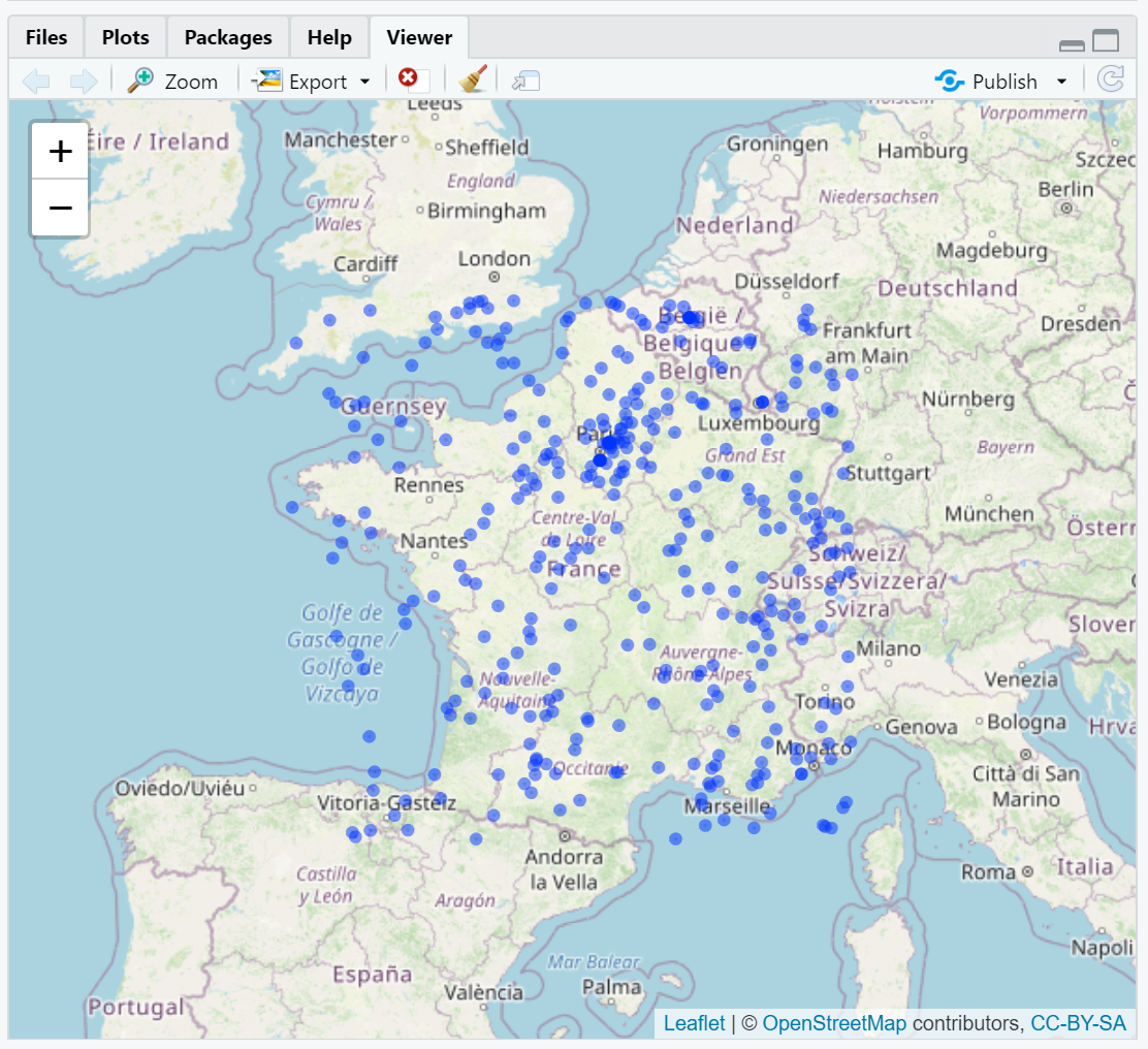
displayAircraftStates()
} else print("You chose to cancel.")
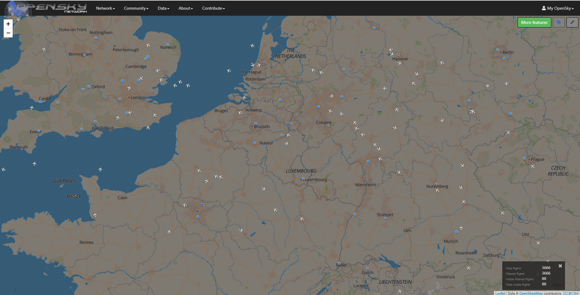
}Now, when you ready to test, enter the command testLiveDataCapture() in the console window. If all goes well, after a minute or so you should see a map like this in the viewer window.
An Infinite Loop to Build Your Live Data Database
Finally, we write a function which will put your R session into an infinite loop. At regular intervals, it will wake up, make a call to the OpenSky API, save the result in your local database, and then go to sleep. On a Windows computer, if you hit “ESC” at any time, it will break out of the infinite loop. If you have a different operating system, you may have to hit the “STOP” button on the RStudio console window to break out of the loop. Copy and paste this code into your sandbox script.
captureLiveDataInfiniteLoop <- function(sleepintervalseconds = 60){
  # launch an infinite loop to capture live data from OpenSkyNetwork
  #https://statisticsglobe.com/stop-running-code-with-keyboard-shortcut-in-r
  print("Capturing data from OpenSkyNetwork. Hit '<Esc>' to exit.")
  query <- 'lomin=-4.935324&lomax=8.384009&lamin=42.423457&lamax=51.179343'
  while (TRUE){
    jsonString <- getOpenSkyData(query)
    dfAircraftStates <-  extractAircraftStates(jsonString)
    appendAircraftStates(dfAircraftStates)
    # Sleep for a period of time
    Sys.sleep(sleepintervalseconds)
  }
}
Run the Infinite Loop Function
When you are ready to collect live data, execute the command captureLiveDataInfiniteLoop(). Let it run for 5 or 10 minutes before hitting the ESC key to exit. That will give you enough data to be interesting for visualization.Then proceed to the next session in this workshop series: “Animate Geographical Data”. If you intend to collect very large amounts of live data, we would not recommend using an SQLite database. It is suitable for small databases. For a mid-sized data collection project, you should consider MySQL or PostGreSQL.
Summary
- Some websites permit access to live or historical data through an application programming interface (API)
- A REST API can be accessed using a URL which includes optional clauses to restrict the search.
- The Open Sky Network has live and archived data on ADS-B transmissions from aircraft around the world.
- Using the
httrpackage in R, you can access the OpenSky API and download ADS-B data. - The OpenSky API returns data as a JSON string.
- With a little data wrangling, using the
dplyrpackage, you can convert the JSON string to a data frame. - Using the
DBI, you can save the data frame of live data to your local SQLite database. - By putting your code in an infinite loop, you can capture and archive live ADS-B data over a period of time.
- SQLite is intended for small databases. MySQL or PostgreSQL are recommended mid-size applications.